Measuring Multicalibration

The Multicalibration Error (MCE) metric quantifies how well a model is multicalibrated across relevant segments (also known as protected groups) of your data. It is used to assess the success of applying a multicalibration algorithm, like MCGrad, by measuring MCE both before and after the multicalibration step. For additional details, see [1].

What is MCE and How Can I Use It?

The Multicalibration Error measures the worst-case noise-weighted calibration error across all segments that can be formed from your specified features. It answers the question: "What is the maximum miscalibration in any segment of my data?"

Key Properties

• $\text{MCE} = 0$ indicates perfect multicalibration;
• Lower values are better;
• Parameter-free - no arbitrary binning decisions required;
• Statistically interpretable - includes p-values.

Quick Start: Computing the MCE

from mcgrad.metrics import MulticalibrationError

mce = MulticalibrationError(
    df=df,
    label_column='label',
    score_column='prediction',
    categorical_segment_columns=['region', 'age_group'],
    numerical_segment_columns=['income']
)

print(f"MCE: {mce.mce:.4f}")
print(f"MDE: {mce.mde:.4f}")
print(f"P-value: {mce.mce_pvalue:.4f}")
print(f"MCE (sigma): {mce.mce_sigma:.2f}")

The output is interpreted as follows:

• mce: The multicalibration error on the absolute scale, in the same units as the predictions (typically in $[0, 1]$).
• mde: The approximate Minimum Detectable Error on the absolute scale. Compare mce to mde: if mce < mde, the observed miscalibration is below the detection threshold for the given sample size.
• mce_pvalue: The p-value for the observed MCE under the null hypothesis of perfect multicalibration. Note that this p-value is not adjusted for multiple testing (see details below).
• mce_sigma: MCE normalized by the standard deviation of the ECCE under perfect calibration. As a practical rule of thumb, values above ~5 are considered significant (see details below).

How Does the MCE Work?

The Multicalibration Error metric is computed in three steps:

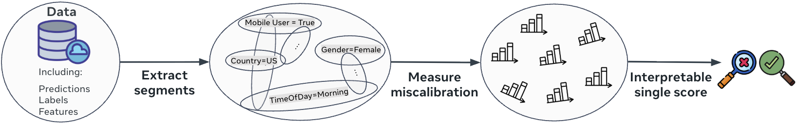
Step 1: Define a Set of Segments

First, specify the collection of segments over which calibration will be assessed. In some applications, segments may be predefined based on domain knowledge (e.g., demographic groups, device types). More commonly, a systematic approach is used:

• Each feature is partitioned into $k$ categories (such as quantiles for numerical features or grouped levels for categorical features).
• All intersections of up to $n$ features are considered, generating a rich set of segments that capture meaningful subpopulations in the data.

Example: In the ad click prediction scenario, to assess multicalibration using the features {market, device_type}, the set of segments would include:

• Segment 0: All samples (global population);
• Segment 1: Users in the US market;
• Segment 2: Users in non-US markets;
• Segment 3: Users on mobile devices;
• Segment 4: Users on desktop devices;
• Segment 5: Users in the US market AND using mobile;
• Segment 6: Users in the US market AND using desktop;
• Segment 7: Users in non-US markets AND using mobile;
• Segment 8: Users in non-US markets AND using desktop.

The number of segments grows exponentially with the number of features. Therefore, the number of features and categories per feature used to identify segments are limited to $n$ and $k$, respectively.

Step 2: Measure Calibration Error Within Each Segment

After defining segments, assess how well the model's predicted probabilities match the observed outcomes within each segment.

For each segment, the [Estimated Cumulative Calibration Error (ECCE)][2] is computed, which captures the sum of deviations between predicted scores and actual labels over any interval of scores in that segment.

Why ECCE?

• ECCE is parameter-free: It does not require arbitrary choices like bin sizes.
• ECCE is statistically interpretable: Its value can be directly related to statistical significance, enabling distinction between genuine miscalibration and random fluctuations.

Example: Continuing with the ad click prediction scenario, for each segment (e.g., "US market AND mobile", "non-US market AND desktop"):

• Samples in the segment are sorted by predicted probability.
• For every possible interval of scores, the cumulative difference between actual clicks and predicted probabilities is calculated.
• The ECCE for the segment is the range of these cumulative differences, normalized by segment size.

Global miscalibrations are also detected, as the first segment represents the entire dataset.

Step 3: Combine Segment Errors Into an Interpretable Single Score

After computing the calibration error (ECCE) for each segment, results are aggregated to produce a single summary metric: the Multicalibration Error (MCE). The MCE is defined as the maximum ECCE across all segments because: practically, the average would be sensitive to the addition of noisier, smaller segments; theoretically, the maximum aligns with the definition of multicalibration as a worst-case guarantee.

Absolute Scale (mce)

The primary MCE metric is on the absolute scale. It is obtained by rescaling the sigma-scale MCE back to the original ECCE units:

$$\text{MCE} = \text{MCE}_\sigma \cdot \hat\sigma_0$$

where $\hat\sigma_0$ is the estimated standard deviation of the global ECCE under perfect calibration. This value is in the same units as the predictions (typically in $[0, 1]$) and represents the absolute magnitude of the worst-case calibration error.

Minimum Detectable Error (mde)

The Minimum Detectable Error (MDE) is on the absolute scale and provides a rough estimate of the smallest calibration error that could be reliably detected given the sample size and properties of the data. Compare mce to mde to assess whether the observed miscalibration is meaningful. It is approximated as:

$$\text{MDE} \approx 5 \cdot \hat\sigma_0$$

where $\hat\sigma_0$ is the global ECCE standard deviation. This approximation assumes the null hypothesis variance, so it is approximate under miscalibration. In practice, MCGrad is typically able to reduce the MCE below the MDE.

Sigma Scale (mce_sigma)

For each segment, the ECCE is normalized by its estimated standard deviation under the null hypothesis of perfect calibration (the "sigma scale"). This accounts for the statistical reliability of each segment and ensures that segments with few samples do not dominate the metric due to noise. The MCE on the sigma scale is the maximum of these normalized errors across all segments:

$$\text{MCE}_\sigma = \max_k \frac{\text{ECCE}_k}{\hat\sigma_k}$$

Higher values indicate stronger statistical evidence for miscalibration. As a practical rule of thumb, we use a threshold of ~5 sigma to flag miscalibration. This is more conservative than typical single-test thresholds because the MCE takes the maximum over many correlated segment-level tests, which inflates the statistic. The 5-sigma threshold is not derived from a formal multiple-testing correction but has proven to work well in practice. This scale depends on dataset properties such as sample size, score distribution, and minority class proportion.

P-value (mce_pvalue)

The p-value represents the probability of the observed MCE under the null hypothesis of perfect multicalibration. It is computed from the distribution of the range of a standard Brownian motion.

Note that this p-value is not adjusted for multiple testing, so the probability of a type I error is somewhat higher in practice. The required adjustment is expected to be small because the hypotheses are highly correlated (many segments overlap).

Relative Scale

For binary classification, a relative scale is also available via mce_relative and mde_relative. These express the MCE and MDE as a percentage of the minority class prevalence ($\text{MCE}_\% = \text{MCE} / \text{prevalence} \times 100$), which can be useful for comparing across datasets with different base rates.

Example: In the ad click prediction scenario, suppose the segment "US market AND mobile" has the highest normalized ECCE. The MCE reflects this value, indicating that this segment is the most miscalibrated and should be the priority for further model improvement.

How Does the MCE Relate to the Theoretical Definition of Multicalibration?

The MCE (sigma scale) metric has a precise mathematical relationship to the theoretical definition of multicalibration, providing a finite-sample estimator of the minimal error parameter in approximate multicalibration.

The Definition of $\alpha$-Multicalibration

The classic definition of multicalibration is straightforward: for every segment $h$ and every predicted probability $p$, the average outcome should match the prediction:

$$\mathbb{E}[Y - f(X) \mid h(X)=1, f(X) = p] = 0.$$

In practice, this condition rarely holds exactly. Therefore, it is relaxed to allow for small error: A predictor $f$ is $\alpha$-multicalibrated with respect to $\mathcal{H}$ if

$$\left| \mathbb{E}\left[h(X) \cdot \mathbf{1}_{f(X) \in [a,b]} \cdot (Y-f(X))\right] \right| \leq \alpha \cdot \tau_h(f,[a,b])$$

for all segments $h \in \mathcal{H}$ and all score intervals $[a,b]$, where:

• $\mathbf{1}_{f(X) \in [a,b]}$ is the interval indicator function;
• $\tau_h(f,[a,b]) = \sqrt{\mathbb{E}[h(X) \cdot \mathbf{1}_{f(X) \in [a,b]} \cdot f(X)(1-f(X))]}$ is the theoretical scale parameter.

This definition captures the intuition that miscalibration should be bounded relative to the statistical uncertainty inherent in each segment and score range.

The Bridge: MCE Directly Estimates $\alpha$

The key insight is that MCE provides a finite-sample estimate of the minimal $\alpha$ for which a model satisfies $\alpha$-multicalibration.

MCE Computation:

$$\text{MCE}(f) = \max_{h \in \mathcal{H}} \frac{\text{ECCE}_h(f)}{\sigma_h(f)}$$

where:

• $\text{ECCE}_h(f)$ measures the range of cumulative calibration differences in segment $h$;
• $\sigma_h(f)$ is the empirical standard deviation of ECCE under perfect calibration.

Scale Parameter Relationship:

The connection between theory and practice lies in the relationship between scale parameters:

• Theoretical scale: $\tau_h(f,[a,b])$ measures population-level uncertainty;
• Empirical scale: $\sigma_h(f)$ estimates finite-sample uncertainty.

Under standard conditions, these are asymptotically equivalent: $\sigma_h(f) \approx \tau_h(f) / \sqrt{n_h}$ where $n_h$ is the segment size.

Mathematical Connection

A predictor $f$ is $\alpha$-multicalibrated with respect to $\mathcal{H}$ if and only if:

$$\text{MCE}(f) \le \alpha \sqrt{n}$$

where $n$ is the sample size.

Proof: Available in Appendix A.1 of MCGrad: Multicalibration at Web Scale.

Why this matters: MCE directly estimates the minimal α for which your model is theoretically guaranteed to be α-multicalibrated across all considered segments.

---

References

[1] Guy, I., Haimovich, D., Linder, F., Okati, N., Perini, L., Tax, N., & Tygert, M. (2025). Measuring multi-calibration. arXiv:2506.11251.

[2] Arrieta-Ibarra, I., Gujral, P., Tannen, J., Tygert, M., & Xu, C. (2022). Metrics of calibration for probabilistic predictions. Journal of Machine Learning Research, 23(351), 1-54.

If you use MCE in academic work, please cite our paper:

@article{guy2025measuring,
  title={Measuring multi-calibration},
  author={Guy, Ido and Haimovich, Daniel and Linder, Fridolin and Okati, Nastaran and Perini, Lorenzo and Tax, Niek and Tygert, Mark},
  journal={arXiv preprint arXiv:2506.11251},
  year={2025}
}