Getting Started
This guide covers the essential steps to begin using MCGrad for multicalibration.
A Basic Multicalibration Workflow
1. Prepare Your Data
MCGrad requires a DataFrame with the following columns:
label— the true binary label for each data point;prediction— the uncalibrated prediction score;categorical_feature_1,categorical_feature_2, ... — optional categorical features that define segments (also known as protected groups);numerical_feature_1,numerical_feature_2, ... — optional numerical features that define segments.
At least one feature is recommended to enable segment identification.
MCGrad requires that predictions:
- are in the range [0, 1];
- do not contain NaN values.
from mcgrad import methods, metrics, plotting
import numpy as np
import pandas as pd

# Generate synthetic data with segment-specific miscalibration
rng = np.random.default_rng(42)
n_samples = 10000

df = pd.DataFrame({
    'country': rng.choice(['US', 'UK'], size=n_samples),
    'content_type': rng.choice(['photo', 'video'], size=n_samples),
    'surface': rng.choice(['feed', 'stories'], size=n_samples),
})

# True probability depends on segments (US and video have higher rates)
df['true_prob'] = 0.5 + 0.15 * (df['country'] == 'US') + 0.1 * (df['content_type'] == 'video')
df['label'] = (rng.uniform(size=n_samples) < df['true_prob']).astype(int)

# Predictions ignore segment effects (miscalibrated)
df['prediction'] = np.clip(rng.uniform(0.3, 0.7, size=n_samples), 0.01, 0.99)
2. Apply MCGrad to Uncalibrated Predictions
MCGrad requires consistency between the categorical and numerical features passed to fit and predict.
Although this example uses the same DataFrame for both methods, in practice the training and prediction DataFrames are typically different. Like other calibration methods (Platt Scaling, Isotonic Regression), MCGrad should be trained on a held-out set (e.g., a validation set) rather than the same data used to train the base model. This prevents overfitting and ensures the calibration generalizes to new data.
# Apply MCGrad
mcgrad = methods.MCGrad()
mcgrad.fit(
    df_train=df,
    prediction_column_name='prediction',
    label_column_name='label',
    categorical_feature_column_names=['country', 'content_type', 'surface'],
    numerical_feature_column_names=[]  # optional, can be empty
)

# Get multicalibrated predictions and add to the DataFrame
df['prediction_mcgrad'] = mcgrad.predict(
    df=df,
    prediction_column_name='prediction',
    categorical_feature_column_names=['country', 'content_type', 'surface'],
    numerical_feature_column_names=[]  # optional, can be empty
)
The multicalibrated predictions are both globally calibrated and multicalibrated:
- Globally calibrated — well-calibrated across all data.
- Multicalibrated — well-calibrated for any segment defined by the features:
- Individual segments like
country=US,country=UK,content_type=photo, ... - Intersections like
country=US AND content_type=photo; - And many more combinations.
- Individual segments like
3. Apply Global Calibration Methods for Comparison
MCGrad includes several global calibration methods for comparison. For example, to apply Isotonic Regression:
# Apply Isotonic Regression
isotonic_regression = methods.IsotonicRegression()
isotonic_regression.fit(
    df_train=df,
    prediction_column_name='prediction',
    label_column_name='label')

# Get globally calibrated predictions and add to the DataFrame
df['prediction_isotonic'] = isotonic_regression.predict(
    df=df,
    prediction_column_name='prediction'
)
See the API Reference for other available global calibration methods.
4. Model Evaluation: The Multicalibration Error Metric
To evaluate multicalibration rigorously, use the MulticalibrationError class, which provides several key attributes:
- Multicalibration Error (MCE): The Multicalibration Error. It measures the largest deviation from perfect calibration over all segments. Access via the
.mceattribute. - MCE Sigma Scale: The Multicalibration Error normalized by its standard deviation under the null hypothesis of perfect calibration. It represents the largest segment error in standard deviations. Conceptually equivalent to a p-value, this metric assesses the statistical evidence of miscalibration. Access via the
.mce_sigmaattribute. - p-value: Statistical p-value measured under the null hypothesis of perfect calibration. This helps determine whether observed miscalibration is statistically significant. Access via the
.mce_pvalueattribute. - Minimum Detectable Error (MDE): The approximate minimum MCE detectable with the dataset. Access via the
.mdeattribute.
# Initialize the MulticalibrationError metric
mce = metrics.MulticalibrationError(
    df=df,
    label_column='label',
    score_column='prediction',
    categorical_segment_columns=['country', 'content_type', 'surface'],
    numerical_segment_columns=[],
)

# Print key calibration metrics
print(f"Multicalibration Error (MCE): {mce.mce:.3f}%")
print(f"MCE Sigma Scale: {mce.mce_sigma:.3f}")
print(f"MCE p-value: {mce.mce_pvalue:.4f}")
print(f"Minimum Detectable Error (MDE): {mce.mde:.3f}%")
See the API Reference for additional evaluation options.
5. Compare Calibration Methods
Compare the multicalibration error metrics across uncalibrated predictions, Isotonic Regression, and MCGrad. Given that the data exhibits segment-specific miscalibration, MCGrad is expected to outperform the other methods.
# Define methods to compare
score_columns = {
    'Uncalibrated': 'prediction',
    'Isotonic': 'prediction_isotonic',
    'MCGrad': 'prediction_mcgrad',
}

# Compute MCE metrics for each method
results = []
for method_name, score_col in score_columns.items():
    mce = metrics.MulticalibrationError(
        df=df,
        label_column='label',
        score_column=score_col,
        categorical_segment_columns=['country', 'content_type', 'surface'],
    )
    results.append({
        'Method': method_name,
        'MCE': round(mce.mce, 2),
        'MCE σ': round(mce.mce_sigma, 2),
        'p-value': round(mce.mce_pvalue, 4),
    })

# Display comparison table
pd.DataFrame(results).set_index('Method')
The output shows that MCGrad significantly reduces the Multicalibration Error compared to both uncalibrated predictions and Isotonic Regression. The p-value for MCGrad (0.0691) indicates no statistically significant evidence of remaining miscalibration.
6. Visualize (Multi)calibration Error
The plotting module provides tools for visualizing (multi)calibration.
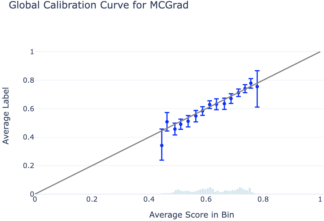
Global Calibration Curves
The global calibration curve displays the average label per score bin. Perfect calibration corresponds to all bin means overlapping with the diagonal line (i.e., the average label equals the average score in each bin). The plot includes 95% confidence intervals for the estimated average label, with a histogram showing the score distribution in the background.
# Plot Global Calibration Curve
fig = plotting.plot_global_calibration_curve(
    data=df,
    score_col="prediction_mcgrad",  # Change this to any model's score column
    label_col="label",
    num_bins=40,
).update_layout(title="Global Calibration Curve for MCGrad", width=700)

fig.show()
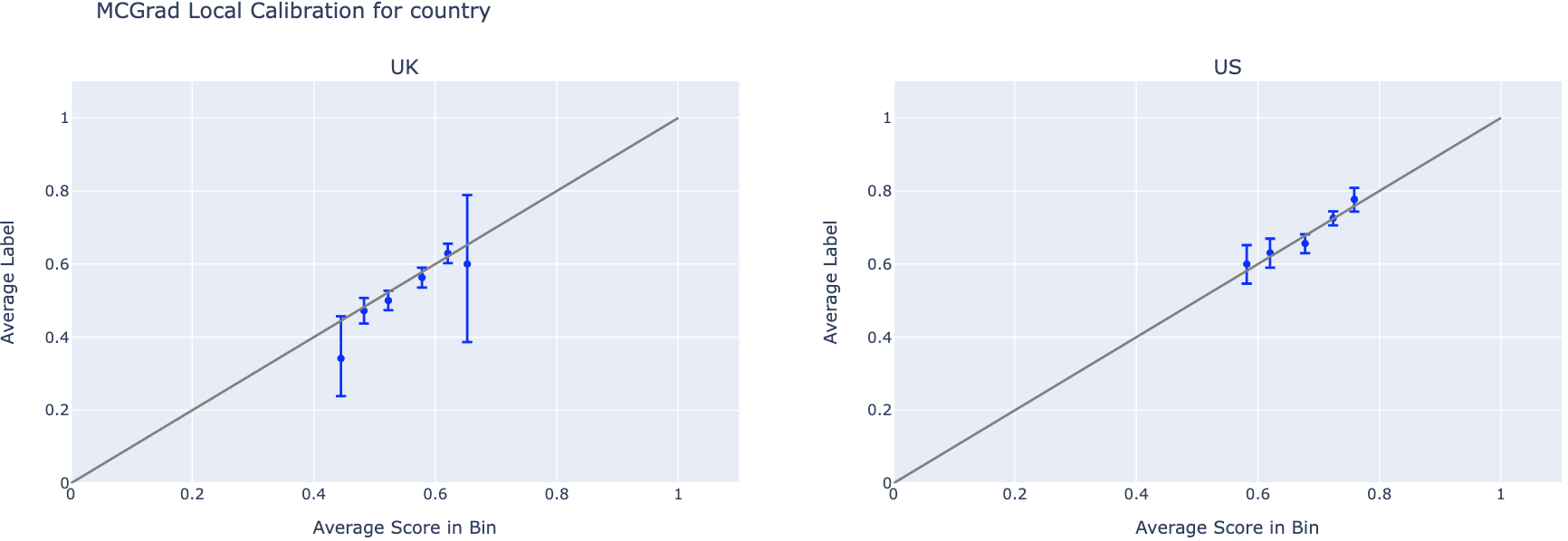
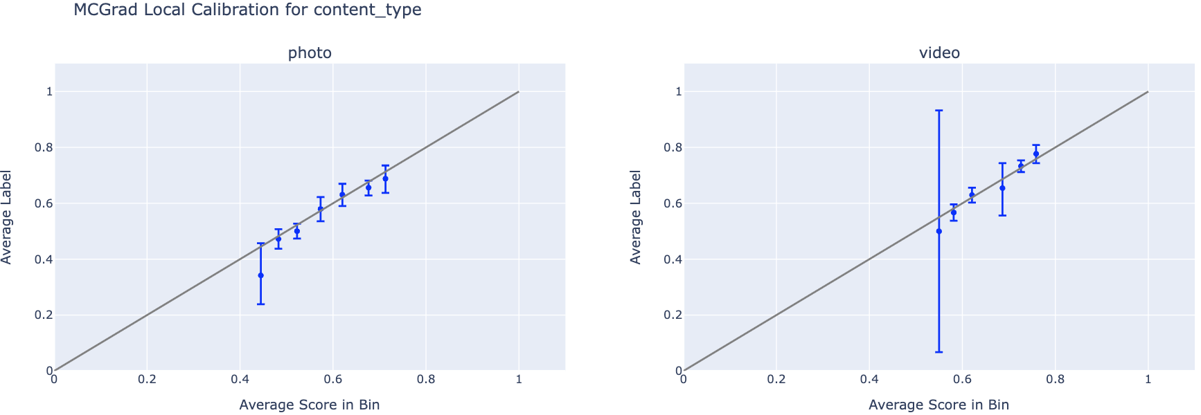
Local Calibration Curves
Local calibration curves display one curve per feature value within a single feature segment. This enables inspection of whether the model is calibrated for specific segments (e.g., country=US, content_type=video), even when it appears calibrated globally.
features_to_plot = ['country', 'content_type']

for feature in features_to_plot:
    n_cats = df[feature].nunique()

    # Plot Local Calibration Curves
    fig = plotting.plot_calibration_curve_by_segment(
        data=df,
        group_var=feature,
        score_col="prediction_mcgrad",  # Change this to any model's score column
        label_col="label",
        n_cols=3,
    ).update_layout(
        title=f"MCGrad Local Calibration for {feature}",
        width=2000,
        height=max(10.0, 500 * (np.ceil(n_cats / 3))),
    )
    fig.show()
See the API Reference for additional visualization options.
Next Steps
- Methodology — Understand how MCGrad works formally.
- Measuring Multicalibration — Understand the Multicalibration Error metric in detail.
- API Reference — Explore all available methods.
- Contributing — Contribute to the project.